
Divide and Conquer Strategies II: Closest Pair of Points
Procedure
Open the Closest Pair of Points – Divide & Conquer Simulation experiment.
Enter the desired number of points N in the input field "Enter no. of points".
Input Constraint: The experiment allows values in the range 2 < N ≤ 20.
If a value outside this range is entered, the system prompts the user to select a valid input.Select the input mode from the Mode dropdown:
Random → Points are generated randomly by the system
Manual → Points are entered manually by the user
Random Mode (Random Generation)
Select Mode = Random.
Click the Load button.
Randomly generated 2D coordinate points are displayed in the Generated Coordinates panel.
The same points are plotted on the visualization canvas with labeled indices.
Manual Mode (User Input)
Select Mode = Manual.
A text input field appears inside the Generated Coordinates panel. Enter the coordinates manually in the format:
x1,y1 x2,y2 x3,y3 ...
Example:
10,20 30,40 50,60Click the Load button.
The manually entered points are validated, displayed in the Generated Coordinates panel, and plotted on the canvas.
Simulation Execution
Once the points are loaded, the navigation controls become active on the right panel.
Click the Auto Play ▾ button to begin the simulation automatically.
Select the execution speed (Slow / Normal / Fast) from the speed dropdown that appears below Auto Play.
Alternatively, use the Next → button to execute the algorithm step-by-step manually.
Use the ← Previous button to revisit earlier steps and analyze recursive divisions and comparisons.
During execution, observe the following steps in the Steps panel on the right:
- Sorting of points based on X-coordinates
- Recursive division of the point set into left and right halves
- Drawing of the Division Line
- Formation of the Strip Region near the dividing line
- Comparison of point pairs inside the strip
- Continuous updates to the current minimum distance (δ)
- The step counter at the top of the Steps panel shows the current step number (e.g., Steps: 5/32), allowing you to track your progress through the algorithm.
Visualization Details
- Observe the following visual indicators on the canvas during execution:
- Blue dashed line → Division Line that splits the point set into left and right halves
- Orange connecting line → The pair of points currently being compared
- Green connecting line → The best (closest) pair found so far
- Labeled points → Each point is displayed with its index for easy identification
- Toggle View (Geometry vs. Recursion Tree)
The simulation provides two distinct ways to observe the algorithm:
- Geometry View (Default): Visualizes the points, division lines, and strip region on the 2D plane.
- Recursion Tree View: Shows the hierarchical breakdown of recursive calls in a binary tree format.
Switching Tabs:
- Use the [ Geometry View | Recursion Tree ] tabs at the top of the visualization area.
- Note: Tab switching is locked during Auto Play to ensure visual synchronization. Stop the autoplay or wait for completion to switch views.
- Recursion Tree Elements
- Nodes: Each box represents a subset of points.
- Labels:
- "Divide" (Blue) → Showing the splitting phase.
- "Base Case" (Purple) → Smallest subproblems (n ≤ 3).
- "Combine" (Green) → Merging results and checking the strip.
- Glow/Pulse: Highlights the active node corresponding to the current step in the log.
- Dual Step Logs
The right panel displays independent logs for each view:
- Geometry Steps: Details geometric operations.
- Recursion Steps: Explains the logic (Divide, Solve, Combine) with educational bullets.
The step counter (e.g., Steps: 5/60) updates dynamically based on the active tab.
- The Legend panel at the bottom-right provides a quick reference:
- 🔵 Division Line / Active Node
- 🟠 Review Pair / Base Case
- 🟢 Best Pair / Completed Node
Facts & Analysis (Runtime Metrics)
- Monitor real-time metrics displayed in the stats bar below the canvas:
- Min Distance → The current minimum distance (δ) found so far
- Comparisons → The total number of distance comparisons performed
- Click the Runtime Metrics button (in the stats bar) to open a detailed modal showing:
- Total Comparisons (D&C) – Number of comparisons made by the Divide & Conquer algorithm
- Total Comparisons (Brute Force) – Number of comparisons a brute force approach would require (N×(N-1)/2)
- Comparisons Saved – The difference, showing how many comparisons were avoided
- Execution Time – The time taken by the D&C algorithm to find the closest pair
Comparison with Brute-Force Approach
Objective of this section:
The objective of this section of the lab is to provide a nuanced comparison of how the Divide and Conquer strategy leads to significant improvements that become clearer as the input size increases. A comparison of both approaches is presented from the perspectives of execution time and number of comparisons made. Observe that the optimal minimum distance is obtained in both approaches, but the Divide and Conquer method achieves this result much more efficiently — with significantly fewer comparisons and faster execution time.
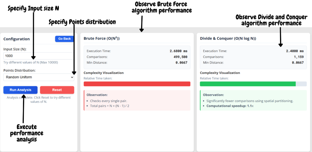
Click the Comparison with Brute-Force approach button (located in the top configuration bar).
A new comparison view opens with its own Configuration panel:
- Enter the input size (N) for scalability analysis (max 10,000)
- Select the point distribution:
- Random Uniform → Points distributed uniformly at random
- Worst Case (Collinear) → All points lie on a straight line
- Best Case (Clusters) → Points form well-separated clusters
Click the Run Analysis button.
Observe and compare the results for both approaches side-by-side:
- Execution Time for Brute Force vs. Divide & Conquer
- Number of Distance Computations for each approach
- Minimum Distance found (should be identical for both)
- Complexity Visualization – relative time bars showing the performance difference
- Computational speedup achieved using Divide & Conquer (displayed as Nx)
- Observations – automatically generated insights for each approach
Click the Reset button to clear the comparison results and try different configurations.
Click the Go Back button to return to the main simulation view.
On the main simulation view, click the Reset button to clear the experiment and perform a new simulation.